
Dustin Lennon
Applied Scientist
dlennon.org
Unlocking TrueType Fonts: Fontforge, Matplotlib, and Partially Ordered Occlusions
This post shows how to merge ttf files and manipulate truetype glyphs.
Dustin Lennon
August 2019
https://dlennon.org/20190819_fontcat
Synopsis
Synopsis
I recently needed to merge the glyphs in two TrueType font files. FontForge, in particular its python extension, appeared to be the tool for the job.
The example below follows the old FontForge documentation. Newer documentation is available here.
The “Barebones” Solution
Pretty simple: sit in a loop and copy A into B; here, k is a glyph index.
import fontforge

Fa = fontforge.open('a.ttf')
Fb = fontforge.open('b.ttf')

for k in Fa:
  if k in Fb:
    continue

  print k
  Fa.selection.select(k)
  Fa.copy()

  Fb.selection.select(k)
  Fb.paste()

Fb.fontname="ico-merged"
Fb.generate("c.ttf")
Fb.generate("c.svg")
Fb.generate("c.eot")
Fb.generate("c.woff")
Going Deeper
Going Deeper
FontForge exposes a Python later that does far deeper than the copy and paste example above. In particular, FontForge provides an object model for character glyphs, and this section provides a walkthrough of how to extract the internal polygonal data and reproduce the glyphs in Matplotlib.
In Figure 1, we show an example codepoint taken from Google’s material icons font.
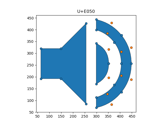
There are a few features to note in Figure 1.
There are three simple polygons, in blue, where ‘simple’ indicates that there are no self-intersections.
Defining these polygons are two classes of points, blue and orange. In the FontForge vernacular, blue points are termed “on-curve”, while orange points are intended to be used as spline knots.
Orange Points and Splines
A bit more should be said about the orange points. The FontForge documentation specifies two scenarios.
First,
If based on cubic splines there should be either 0 or 2 off-curve points between every two on-curve points. If there are no off-curve points then we have a line between those two points. If there are 2 off-curve points we have a cubic bezier curve between the two end points.
Second,
If based on quadratic splines things are more complex. Again, two adjacent on-curve points yield a line between those points. Two on-curve points with an off-curve point between them yields a quadratic bezier curve. However if there are two adjacent off-curve points then an on-curve point will be interpolated between them. (This should be familiar to anyone who has read the truetype ‘glyf’ table docs).
The first case is relatively simple and, as Google’s material icons rely on quadratic splines, we focus only on the second case.
If we assume that there is always at least one blue point; that is, one on-curve point, we can loop through the points using the following state diagram:
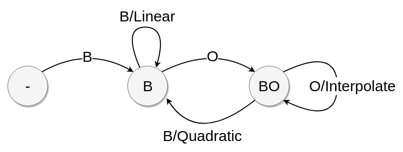
In Figure 2, ‘B’ indicates a blue, on-point coordinate whereas ‘O’ is an orange, not on-point coordinate. The state labels are
- ‘-’ indicates the initial start state where the first point processed in an on-point curve, the one we assumed to exist earlier.
- ‘B’ and ‘BO’ are best though of as prefixes in the sense that the on-point status of the next point processed will determine some action.
Constructing a matplotlib Path
Constructing a matplotlib Path
Such a state diagram is easily coded up.
def _quadratic_verts_codes(pts):
  """
  Extract the components of a matplotlib.path.Path from a list of (x,y) coordinates.
  """
  curve = []  # keep track of our prefixes
  codes = []
  verts = []

  state = _State.INIT
  for i,pt in enumerate(pts):
    curve.append( pt )
    if state == _State.INIT:
      if pt.on_curve:
        state = _State.START
      else:
        raise ShapeError("contour should start with a point on the curve")
    elif state == _State.START:
      if pt.on_curve:
        _segment_linear(curve, verts, codes)
        state = _State.START
      else:
        state = _State.Q
    elif state == _State.Q:
      if pt.on_curve:
        _segment_quadratic(curve, verts, codes)
        state = _State.START
      else:
        _segment_interpolate(curve, verts, codes)
        state = _State.Q

  return (verts, codes)
The linear interpolation method is straightforward, so we include only the quadratic and interpolate pieces below.
In the quadratic case, we know we are processing a B-O-B sequence of points as a quadratic spline. The (matplotlib documentation)[https://matplotlib.org/3.1.1/api/path_api.html#matplotlib.path.Path.codes] states:
The list of codes in the Path as a 1-D numpy array. Each code is one of STOP, MOVETO, LINETO, CURVE3, CURVE4 or CLOSEPOLY. For codes that correspond to more than one vertex (CURVE3 and CURVE4), that code will be repeated so that the length of self.vertices and self.codes is always the same.
Thus, we process B-O-B as a quadratic spline, and the second B becomes the new prefix.
def _segment_quadratic(curve, verts, codes):
  _verts = [(p.x, p.y) for p in curve]
  if len(_verts) == 3:
    _codes = [Path.MOVETO, Path.CURVE3, Path.CURVE3]
  else:
    raise ValueError("_segment_quadratic")

  codes.extend( _codes )
  verts.extend( _verts )
  curve[:] = curve[-1:]
For the interpolate case, we know we are procssing a B-O-O sequence of points. For quadratic spline contours, a consecutive pair of O’s requires an interpolation: there is a ‘b’ to be computed between each ‘O.’ Thus, B-O-O becomes B-O-b-O. We process B-O-b with our quadratic code and, finally, b-O becomes the new prefix.
def _segment_interpolate(curve, verts, codes):
  a,b,c = curve
  mbc   = fontforge.point((b.x+c.x)/2., (b.y+c.y)/2., 1L)
  _segment_quadratic([a,b,mbc], verts, codes)
  curve[:] = [mbc,c]
Oriented Contours and Holes
Oriented Contours and Holes
For simple polygons, such as those in Figure 1, the problem of extracting a polygon from a collection of blue and orange points is solved. This section introduces the idea of holes in polygons, and we discuss how to handle this more general case.
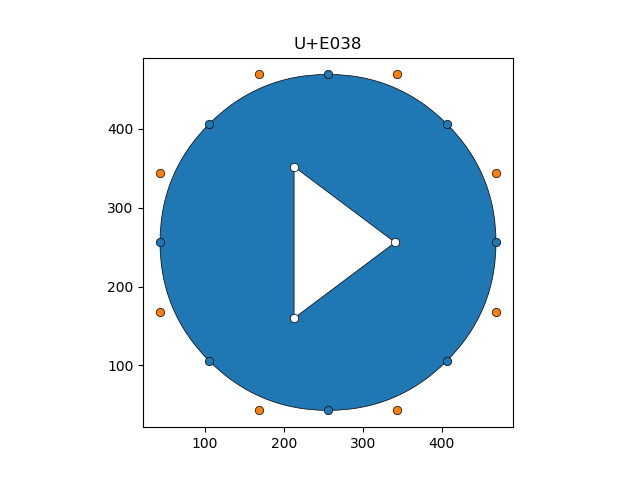
Figure 3 shows a polygon with a hole. There are two ways to process this image. One is that there is a triangular hole in the circle; the other, that a white triangle has been drawn on top of a circle. The white points are suggestive of the latter interpretation.
In fact, the glyph object model for U+E038 would store two contours. One for the circle and a second for the triangle. The distinction between these contours is their orientation. In particular, the points defining the circle are stored clockwise whereas those for the triangle are stored counter-clockwise (ccw), and the long-standing convention is that ccw indicates a hole.
Given only polygons and their orientations, then, we might hope that plotting them would be straightforward. A naive strategy might be to plot the clockwise polygons first and then plot the counter-clockwise polygons on top. Figure 4 shows how this strategy might fail.
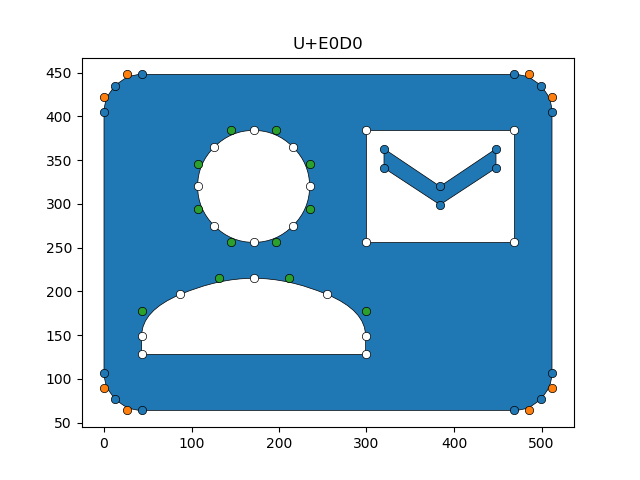
In particular, Figure 4 shows a polygon with several holes, and one of the holes contains a second polygon, a chevron, which is cw-oriented and also needs to be plotted in front of the rectangle. Following the naive strategy, the chevron would be invisible: it would be plotted behind the rectangular hole. To address the issue of occlusions, we need a more satisfactory approach.
One possibility is to consider all the polygons in the context of containment: if, as a point set, \(P_2 \subset P_1\), that is, if \(P_1\) contains \(P_2\), then we should draw \(P_1\) before drawing \(P_2\). The only complication is if, say, \(P_2\), is a subset of multiple other polygons. In Figure 4, this is the case for the chevron: as a point set, it is contained by both the white rectangle and the blue matte background.
The idea of using subsets to induce a (partial) ordering is naturally captured by a tree structure. See, Figure 5, for an example.

We describe an algorithm for producing such a data structure in the next section.
Partially Ordered Occlusions: Building the Forest
The algorithm described in this section constructs the partially ordered occlusions forest. In general, this forest will be a collection of trees.
First, note that each node will be identified with a polygon from the glyph.
To begin, we start with a preprocessing step where, for each polygon, we identify its complete set of ancestors and descendants. Our construction starts from the leaf nodes and proceeds to the root of the tree. We identify leaf nodes, remove them from consideration, and repeat, noting that the subsequent step necessarily identifies parental candidates of current leaves.
The code is mostly bookkeeping:
def construct(self):
  for i,pi in enumerate(self.polygons):
    for j,pj in enumerate(self.polygons[(i+1):], start=i+1):
      if not pi.intersects(pj):
        pi.ignored_idx.add(j)
        pj.ignored_idx.add(i)
        continue

      if pi.contains(pj):
        pi.descendent_idx.add(j)
        pj.ancestor_idx.add(i)
      elif pj.contains(pi):
        pj.descendent_idx.add(i)
        pi.ancestor_idx.add(j)
      else:
        raise NotImplementedError("polygons intersect but no proper subset relation exists")
  self.reduce()

def reduce(self):
  polygon_idx = range(len(self.polygons))

  while any(polygon_idx):
    for i in polygon_idx:
      if i is None:
        continue
      pi  = self.polygons[i]
      dmi = pi.descendent_idx - pi.ignored_idx
      if len(dmi) == 0:
        polygon_idx[i]  = None

        for j in pi.ancestor_idx:
          self.polygons[j].ignored_idx.add(i)

        for j in pi.descendent_idx:
          pj        = self.polygons[j]
          if pj.parent is not None:
            continue

          pj.parent = pi
          self.polygons[i].children.add( pj )
The complete code is available here, and the font file here.