
Dustin Lennon
Applied Scientist
dlennon.org
statsmodels
pystan
linear regression
bayesian analysis
non-informative priors
[GH07] Figure 3.1: Mothers' education and children's test scores
This notebook replicates results in GH07, section 3.1, using (a) the statsmodels package and (b) the pystan package.
Dustin Lennon
September 2019
https://dlennon.org/20190918_stan001
September 2019
Simple Linear Regression Using a Bayesian Model
Simple Linear Regression Using a Bayesian Model
Simple Linear Regression Using a Bayesian Model
We replicate the results of a classical simple linear regression using a bayesian model with non-informative priors. This is effectively “Hello, World” using the PyStan package.
import matplotlib.pyplot as plt
from matplotlib.lines import Line2D as Line2D
from matplotlib.figure import Figure as Figure
import os
import numpy as np
import pandas as pd
import statsmodels.api as sm
import pystan
import arviz as az
# pystan model cache
import sys
sys.path.append(r"./cache/mc-stan")
import model_cache
Dataset
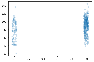
We replicate GH07, Figure 3.1. This uses the mother’s education and children’s test scores dataset.
# Load data
df = pd.read_stata("~/Workspace/Data/ARM/child.iq/kidiq.dta")
df.head()
| kid_score | mom_hs | mom_iq | mom_work | mom_age | |
|---|---|---|---|---|---|
| 0 | 65 | 1.0 | 121.117529 | 4 | 27 |
| 1 | 98 | 1.0 | 89.361882 | 4 | 25 |
| 2 | 85 | 1.0 | 115.443165 | 4 | 27 |
| 3 | 83 | 1.0 | 99.449639 | 3 | 25 |
| 4 | 115 | 1.0 | 92.745710 | 4 | 27 |
# data
x   = df['mom_hs']
y   = df['kid_score']

# jitter (for scatterplot)
np.random.seed(1111)
xj  = x + np.random.uniform(-0.03,0.03,size=len(x))
# Scatterplot
fig = plt.figure()
ax = fig.gca()
pc = ax.scatter( *[xj,y], alpha=0.25, ec=None, lw=0)
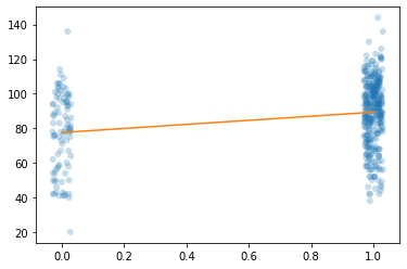
Baseline Model: Classical OLS / Simple Linear Regression
# OLS fit
X = np.column_stack(np.broadcast_arrays(1,x))
model = sm.OLS(y, X)
results = model.fit()
print(results.summary())
OLS Regression Results
==============================================================================
Dep. Variable:              kid_score   R-squared:                       0.056
Model:                            OLS   Adj. R-squared:                  0.054
Method:                 Least Squares   F-statistic:                     25.69
Date:                Wed, 03 Mar 2021   Prob (F-statistic):           5.96e-07
Time:                        15:05:26   Log-Likelihood:                -1911.8
No. Observations:                 434   AIC:                             3828.
Df Residuals:                     432   BIC:                             3836.
Df Model:                           1
Covariance Type:            nonrobust
==============================================================================
                 coef    std err          t      P>|t|      [0.025      0.975]
------------------------------------------------------------------------------
const         77.5484      2.059     37.670      0.000      73.502      81.595
x1            11.7713      2.322      5.069      0.000       7.207      16.336
==============================================================================
Omnibus:                       11.077   Durbin-Watson:                   1.464
Prob(Omnibus):                  0.004   Jarque-Bera (JB):               11.316
Skew:                          -0.373   Prob(JB):                      0.00349
Kurtosis:                       2.738   Cond. No.                         4.11
==============================================================================

Notes:
[1] Standard Errors assume that the covariance matrix of the errors is correctly specified.
# Add a trend line based on OLS fit
yhat = results.predict([[1,0],[1,1]])
trend = Line2D([0,1], yhat, color='#ff7f0e')
ax.add_artist(trend)
ax.figure
Non-informative Bayesian Model
model_code = """
    data {
        int<lower=0> N;
        vector[N] x;
        vector[N] y;
    }
    parameters {
        real alpha;
        real beta;
        real<lower=0> sigma;
    }
    model {
        y ~ normal(alpha + beta * x, sigma);
    }
"""

mod = model_cache.retrieve(model_code)
Using cached StanModel
model_data = {
    'N' : len(x),
    'x' : x,
    'y' : y
}

fit = mod.sampling(data=model_data, iter=1000, chains=4, seed=4792)
print(fit)
Inference for Stan model: anon_model_6fddc89ca61cc8fa76fc51c1448e28ab.
4 chains, each with iter=1000; warmup=500; thin=1;
post-warmup draws per chain=500, total post-warmup draws=2000.
mean se_mean sd 2.5% 25% 50% 75% 97.5% n_eff Rhat
alpha 77.56 0.07 1.95 73.98 76.11 77.48 78.93 81.49 895 1.0
beta 11.76 0.07 2.21 7.27 10.25 11.86 13.33 15.95 954 1.0
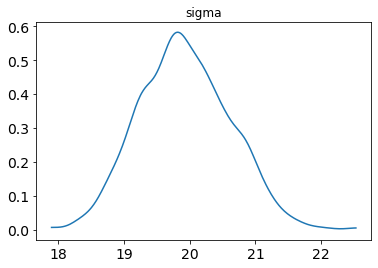
sigma 19.93 0.02 0.69 18.65 19.43 19.9 20.39 21.31 1106 1.0
lp__ -1511 0.04 1.09 -1514 -1511 -1511 -1510 -1510 750 1.0
Samples were drawn using NUTS at Wed Mar 3 15:05:26 2021.
For each parameter, n_eff is a crude measure of effective sample size,
and Rhat is the potential scale reduction factor on split chains (at
convergence, Rhat=1).
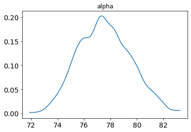
Posterior Samples
samp = fit.extract(permuted=True)

def posterior_plot(samp, k):
    fig = plt.gcf()
    ax = fig.gca()
    az.plot_kde(samp[k], ax = ax)
    ax.set_title(k)
    ax.figure
posterior_plot(samp, 'alpha')
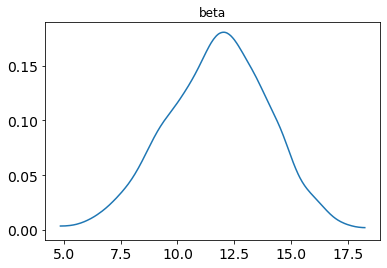
posterior_plot(samp, 'beta')
posterior_plot(samp, 'sigma')
Bibliography
Bibliography
Bibliography
[GH07] Gelman, A., and Hill, J. (2007). Data Analysis Using Regression and Multilevel/Hierarchical Models. Chapter 3.