Dustin Lennon
Applied Scientist
dlennon.org
An Introduction to pytrope.psycopg2_extras
This notebook serves as an introduction to the pytrope.psycopg2_extras package.
Dustin Lennon
October 2019
https://dlennon.org/20191009_pytrope
An Introduction to Pytrope.Psycopg2_Extras
An Introduction to Pytrope.Psycopg2_Extras
This module provides helper two objects, DatabaseManager and SqlQueryManager. The former provides a simple copyto method for copying pandas.DataFrames to PostgreSQL tables; and a more general, dbexecute method, for sending arbitrary SQL queries to a PostgreSQl server and returning any recordset provided as a pandas.DataFrame. All communication with the PostgreSQL server is via the python package, psycopg2.
SqlQueryManager relies on a DatabaseManager to provide a toolset for iterative, incremental SQL query construction. It effectively manages partial query dependencies via a dynamically constructed with_clause.
source code on github
The source repository is hosted on github, available at https://github.com/dustinlennon/pytrope.
environment setup
This code in this section is mostly contextual: Jupyter configuration, Python imports, matplotlib tweaks, and loading a small dataset.
import matplotlib
import matplotlib.pyplot as plt
import matplotlib.dates as mdates

import pandas as pd
import datetime

import pytrope.psycopg2_extras
the dataset
This dataset is a sample, by user, from an Uber Analyst Exercise based on a larger collection of trip records.
# Load some data
kw = {
  'header' : 0,
  'names' : ['trip_date', 'rider_id', 'trip_id', 'city_id'],
  'converters' : {
    'trip_date' : lambda x: datetime.datetime.strptime(x, "%Y-%m-%d").date()
  }
}

url = r"https://dlennon.org/assets/data/b1bfaf29365c192946f979a4d325ef8b.bz2"
trips_data = pd.read_csv(url, **kw)
DatabaseManager
DatabaseManager
The database manager requires a data source name (DSN) for a configured PostgreSQL database. See the PostgreSQL connection string documentation for more information. Simply pass the DSN string to the DatabaseManager constructor. Note that we include a search_path in the DSN below to set the schema.
# Set up the DatabaseManager object
dsn = r"host=192.168.1.102 port=5432 dbname=sandbox user=deploy sslmode=require options=-c\ search_path=uber"
dbm = pytrope.psycopg2_extras.DatabaseManager(dsn)
the copyto method
The copyto method copies a pandas DataFrame to a table in the database. If the table exists, it will be dropped and re-created.
# [pytrope.psycopg2_extras] copy the trips_data pandas.DataFrame to a PostgreSQL table, 'trips'
dbm.copyto(trips_data, 'trips')
the dbexecute method
The dbexecute method allows arbitrary SQL queries to be passed to the database. Any records returned are cast to pandas DataFrames.
# [pytrope.psycopg2_extras] query the response
v = dbm.dbexecute("SELECT COUNT(*) FROM trips")
v
| count | |
|---|---|
| 0 | 123 |
SqlQueryManager
SqlQueryManager
Most queries are built up from simpler components. SqlQueryManager ingests these simpler components, which may refer recursively to previously ingested components, and includes a relevant with_clause for all final queries. SqlQueryManager also maintains partial queries as cached DataFrame’s, enabling pandas operations on the python side. This makes it far easier to iterative construct queries.
# Set up the SqlQueryManager object
sqm = pytrope.psycopg2_extras.SqlQueryManager(dbm)
# Create a partial query, 'rider_date', and add it to the SqlQueryManager
rider_date = """
  SELECT
    rider_id,
    MIN(trip_id) as trip_id,
    trip_date
  FROM
    trips
  GROUP BY
    rider_id, trip_date
"""
sqm.set_pq('rider_date', rider_date, order_by = ['rider_id', 'trip_date'])
# rider_date is now available as an attribute of sqm, a pandas.DataFrame
sqm.rider_date.head()
| rider_id | trip_id | trip_date | |
|---|---|---|---|
| 0 | 0 | 3494 | 2019-06-13 |
| 1 | 0 | 5058 | 2019-06-18 |
| 2 | 0 | 5968 | 2019-06-21 |
| 3 | 1 | 4737 | 2019-06-17 |
| 4 | 2 | 4961 | 2019-06-18 |
a parameterized sql
Below, we use the usual python formatting tools to parameterize a SQL query.
# Create a second partial query, 'full_date_range', and add it to the SqlQueryManager
period_len  = 7
start_date  = datetime.date(2019, 6, 1)
end_date    = datetime.date(2019, 8, 5)

full_date_range = """
  SELECT
    DATE(generate_series) AS cur_date,
    DATE(generate_series) - INTEGER '{pmau_start}' as pmau_start,
    DATE(generate_series) - INTEGER '{pmau_end}' as pmau_end,
    DATE(generate_series) - INTEGER '{mau_start}' as mau_start,
    DATE(generate_series) - INTEGER '{mau_end}' as mau_end
  FROM
    generate_series('{start_date}'::timestamp, '{end_date}'::timestamp, '1 day')
  """.format(**{
    'pmau_start' : 2*period_len,
    'pmau_end': period_len + 1,
    'mau_start' : period_len,
    'mau_end' : 1,
    'start_date': start_date,
    'end_date' : end_date
})
sqm.set_pq('full_date_range', full_date_range, order_by = ['cur_date'])
# 'full_date_range' is available as a component of the SQL WITH clause
print( sqm.with_clause() )
WITH
rider_date AS (
  SELECT
    rider_id,
    MIN(trip_id) as trip_id,
    trip_date
  FROM
    trips
  GROUP BY
    rider_id, trip_date
),
full_date_range AS (
  SELECT
    DATE(generate_series) AS cur_date,
    DATE(generate_series) - INTEGER '14' as pmau_start,
    DATE(generate_series) - INTEGER '8' as pmau_end,
    DATE(generate_series) - INTEGER '7' as mau_start,
    DATE(generate_series) - INTEGER '1' as mau_end
  FROM
    generate_series('2019-06-01'::timestamp, '2019-08-05'::timestamp, '1 day')
  )
a cleaner sql
The subsequent query is kept simple as it can reference previous queries, namely ‘full_date_range’ and ‘rider_date’ through the SqlQueryManager. We can focus on components rather than wading through a nested visual mess.
# create the pre-aggregated, per-(date,user) 'mau', and add it to the SqlQueryManager
mau_bins = """
  SELECT DISTINCT
    D.cur_date,
    R.rider_id
  FROM
    full_date_range AS D
  CROSS JOIN
    rider_date AS R
  WHERE
    D.mau_start <= R.trip_date AND R.trip_date <= D.mau_end
"""
sqm.set_pq('mau_bins', mau_bins, order_by = ['cur_date'])
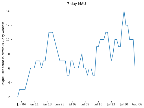
back to pandas
We can also run aggregations and analytics on the python side. Below, we deploy a pandas groupby method on the DataFrame extracted in the previous query.
# Plot of 7-day MAU, "WAU", over time
fig = plt.gcf()
fig.clf()
ax = fig.gca()

sqm.mau_bins.groupby('cur_date').count().plot(ax=ax, legend=False)
ax.xaxis.set_major_locator(mdates.WeekdayLocator())
ax.xaxis.set_major_formatter(mdates.DateFormatter('%b %d'))
ax.set_xlabel('')
ax.set_ylabel('unique user count in previous 7-day window')
ax.set_title('7-day MAU');