Adaptive Rejection Sampling

This work was originally published as an Inferentialist blog post.
Abstract
Adaptive rejection sampling is a statistical algorithm for generating samples from a univariate, log-concave density. Because of the adaptive nature of the algorithm, rejection rates are often very low.
The exposition of this algorithm follows the example given in Davison’s 2008 text, “Statistical Models.”
Algorithm
The algorithm is fairly simple to describe:
- Establish a set of fixed points and evaluate the log-density, \(h\), and derivative of the log-density on the fixed points.
- Use these function evaluations to construct a piecewise-linear, upper bound for the log-density function, \(h_+\), via supporting tangent lines of the log-density at the fixed points.
- Let \(g_+ = \exp(h_+)\). Because of the piecewise-linear construction of \(h_+\), \(g_+\) is piecewise-exponential, sampling \(Y \sim g_+\) is straightforward.
- Pick \(U \sim
\mbox{Unif}(0,1)\).
If \(U \leq \exp \left( h(Y) - h_+(Y) \right)\), accept \(Y\); else, draw another sample from \(g_+\). - For any \(Y\) rejected by the above criteria, \(Y\) may be added to the initial set of fixed points and the piecewise-linear upper bound, \(h_+\), adaptively updated.
An Example
We apply the algorithm to Example 3.22 in Davison. Here we specify a log-concave density function. Note \(\exp(h)\) is the density, and \(h\) is the concave log-density:
\[ h(y) = ry - m \log(1 + \exp(y)) - \frac{(y-\mu)^2}{2\sigma^2} + c \]
where \(y\) is real valued, \(c\) is a constant such that the integral of \(\exp(h)\) has unit area, \(r = 2\), \(m=10\), \(\mu = 0\), and \(\sigma^2 = 1\).
R Code
First, define the function, h, and its derivative, dh.
## Davison, Example 3.22
params.r = 2
params.m = 10
params.mu = 0
params.sig2 = 1

## the log of a log-convex density function
ymin = -Inf
ymax = Inf
h = function(y){
    v = params.r*y - params.m * log(1+exp(y)) - (y-params.mu)^2/(2*params.sig2) # plus normalizing const
    return(v)
}

## derivative of h
dh = function(y)
{
    params.r - params.m * exp(y) / (1 + exp(y)) - (y-params.mu)/params.sig2
}
Define the function that computes the intersection points of the supporting tangent lines. Suppose \(y_1, \dots, y_k\) denotes the fixed points. Then,
\[ z_j = y_j + \frac{h(y_j) - h(y_{j+1}) + (y_{j+1} - y_j) h'(y_{j+1})}{h'(y_{j+1}) - h'(y_j)} \]
## compute the intersection points of the supporting tangent lines
zfix = function(yfixed)
{
    yf0 = head(yfixed, n=-1)
    yf1 = tail(yfixed, n=-1)
    zfixed = yf0 + (h(yf0) - h(yf1) + (yf1 - yf0)*dh(yf1)) / (dh(yf1) - dh(yf0))
    return(zfixed)
}
and the piecewise-linear upper bound,
\[ h_+(y) = \begin{cases} h(y_1) + ( y - y_1 ) h'(y_1) & y \leq z_1, \\ h(y_{j}) + ( y_{j+1} - y_j ) h'(y_{j+1}) & z_{j} \leq y \leq z_{j+1} \\ h(y_{k}) + ( y - y_k ) h'(y_{k}) & z_{k} \leq y \end{cases} \]
## evalutate the unnormalized, piecewise-linear upper-bound of the log-density
hplus = function(y, yfixed)
{
    res = rep(0, length(y))
    zfixed = zfix(yfixed)

    piecewise.idx = findInterval(y, c(ymin, zfixed, ymax))
    npieces = length(zfixed) + 2
    for(pidx in 1:npieces){
        yp = y[piecewise.idx == pidx]
        xx = h(yfixed[pidx]) + (yp - yfixed[pidx])*dh(yfixed[pidx])
        res[piecewise.idx == pidx] = xx
    }
    return(res)
}
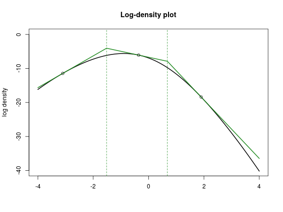
In the following plot, \(h\) is shown in black, and \(h_+\) is in green. The black circles are \((y_i, h(y_i))\), and the dashed green vertical lines are \(z_i\).

We implement a vectorized function to compute the (normalized) CDF of \(g_+ = \exp(h_+)\):
\[ \begin{align*} G_+(y) & = \int_{-\infty}^y \exp(h_+(x)) dx \\ & = \int_{-\infty}^{\min\{z_1,y\}} \exp(h_+(x)) dx \\ & \qquad + \int_{z_1}^{\min\{z_2,\max\{y, z_1\}\}} \exp(h_+(x)) dx \\ & \qquad + \cdots \\ & \qquad + \int_{z_{k-1}}^{\min\{z_k,\max\{y, z_{k-1}\}\}} \exp(h_+(x)) dx \\ & \qquad + \int_{z_k}^{\max\{z_k,y\}} \exp(h_+(x)) dx \end{align*} \]
In particular, the above formulation means that we can precompute \(G_+(z_i)\) which means it is only necessary to compute the last, non-zero integral for each \(y\).
gplus.cdf = function(vals, yfixed)
{
    # equivalently:  integrate(function(z) exp(hplus(z, yfixed)), lower=-Inf, upper = vals)

    zfixed = zfix(yfixed)

    zlen = length(zfixed)
    pct = numeric(length(vals))
    norm.const = 0
    for(zi in 0:zlen) {
        if(zi == 0)
        {
            zm = -Inf
        } else {
            zm = zfixed[zi]
        }

        if(zi == zlen)
        {
            zp = Inf
        } else {
            zp = zfixed[zi+1]
        }

        yp = yfixed[zi+1]
        ds = exp(h(yp))/dh(yp) * ( exp((zp - yp)*dh(yp)) - exp((zm - yp)*dh(yp)) )

        cidx = zm < vals & vals <= zp
        hidx = vals > zp

        pct[cidx] = pct[cidx] + exp(h(yp))/dh(yp) * ( exp((vals[cidx] - yp)*dh(yp)) - exp((zm - yp)*dh(yp)) )
        pct[hidx] = pct[hidx] + ds

        norm.const = norm.const + ds
    }

    l = list(
            pct = pct / norm.const,
            norm.const = norm.const
        )
    return(l)
}
Next, we write a function to sample from \(g_+\). This proceeds via a probability integral transform, inverting realizations from a \(\mbox{Unif}(0,1)\) distribution. Using the previous sum-of-integrals formulation for \(G_+\), this requires a search across \(\{ G_+(z_1), \cdots G_+(z_{k-1}) \}\) and then inverting a single integral.
## sample from the gplus density
gplus.sample = function(samp.size, yfixed)
{
    zfixed = zfix(yfixed)
    gp = gplus.cdf(zfixed, yfixed)
    zpct = gp$pct
    norm.const = gp$norm.const
    ub = c(0, zpct, 1)

    unif.samp = runif(samp.size)

    fidx = findInterval(unif.samp, ub)
    num.intervals = length(ub) - 1
    zlow = c(ymin, zfixed)
    res = rep(NaN, length(unif.samp))
    for(ii in 1:num.intervals)
    {
        ui = unif.samp[ fidx == ii ]

        if(length(ui) == 0)
        {
            next
        }

        ## Invert the gplus CDF
        yp = yfixed[ii]
        zm = zlow[ii]
        tmp = (ui - ub[ii]) * dh(yp) * norm.const / exp(h(yp)) + exp( (zm - yp)*dh(yp) )
        tmp = yp + log(tmp) / dh(yp)
        res[ fidx == ii ] = tmp
    }
    return(res)
}
Results
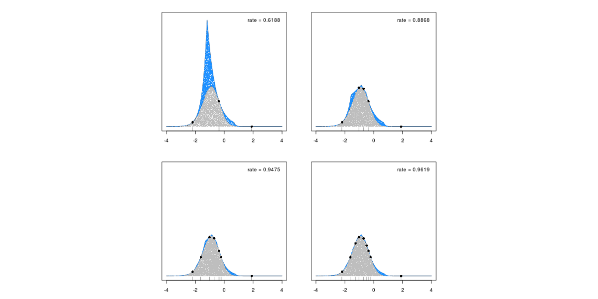
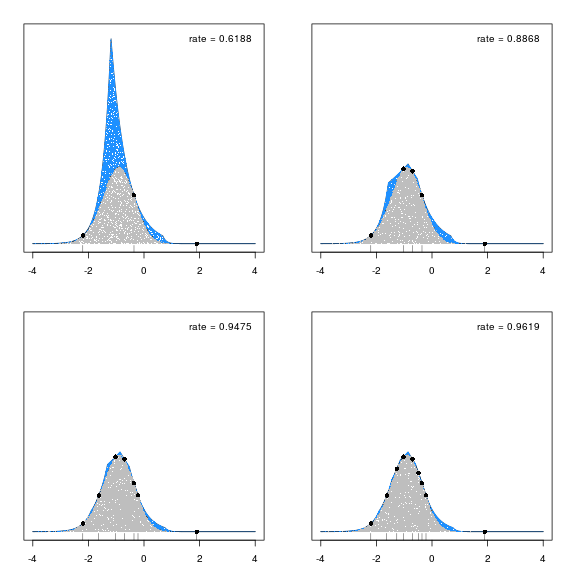
The results are impressive. It takes only a handful of fixed points to reach an acceptance rate that exceed 95%. The figure below shows this convergence. In each plot, 10000 samples are taken from \(g_+\). Blue dots show rejected samples, and gray dots show samples from the target density, \(g\). After each experiment, two of the rejected points are chosen as new fixed points. The black dots, and corresponding rug plot, indicate these fixed points. With only 9 fixed points, the acceptance rate is 96%.
