Numerical Linear Algebra: QR, Hessenberg, and Schur

This post follows Golub and Van Loan, introducing Householder relections and Givens rotations, then using these tools to sketch out implementations of QR, Hessenberg, and Schur decompositions.
import numpy as np
np.set_printoptions( precision=3, linewidth = 132, suppress = True )
First, create some test data:
# Set dimensions and create identity matrices
m,n = (8,6)
I_m = np.identity(m)
I_n = np.identity(n)

# Seed the RNG.
rng = np.random.default_rng(111)

# A: a "tall" m x n matrix
data = rng.negative_binomial(10, 0.25, size=m*n)
A0 = np.array(data, dtype=np.float64).reshape((m,n))

# B: a square n x n matrix
data = rng.negative_binomial(10, 0.25, size=n*n)
B0 = np.array(data, dtype=np.float64).reshape((n,n))
QR factorization
house computes a Householder matrix. This takes a vector
and returns a matrix that zeros out the trailing portion.
def house(x):
  """
  Golub and Van Loan, 3rd Ed.
  Algorithm 5.1.1
  """
  n = len(x)
  sigma = x[1:] @ x[1:]
  v = np.concatenate([[1], x[1:]])

  if sigma == 0:
    beta = 0
  else:
    mu = np.sqrt(x[0]**2 + sigma)
    if x[0] <= 0:
      v[0] = x[0] - mu
    else:
      v[0] = -sigma / (x[0] + mu)
    beta = 2 * v[0]**2 / (sigma + v[0]**2)
    v = v/v[0]

  return(v, beta)
When we apply the above to the first column of A, we
obtain a vector that has zeros in all but the first component.
# A householder matrix to zero out elements of the first column of A

# Let `x0` be the first column of A
x0 = A0[:,0].copy()

# Compute the householder matrix
v, beta = house(x0)
P0 = (I_m - beta * np.outer(v,v))

# Its effect: zeroes!
P0 @ x0
array([102.113, 0. , 0. , 0. , -0. , -0. , -0. , 0. ])A second application can be applied, iteratively, to the next column of A. In the context of a QR factorization, it need only concern itself with zeros below the diagonal.
P1 = np.identity(m)

# Let `x1` be the next column of A.
x1 = A0[:,1].copy()

# A Householder matrix to introduce zeros below the diagonal in the second column.  At the
# second iteration, we'll be working with P0 @ x:
v1, b1 = house((P0 @ x1)[1:m])
P1[1:m, 1:m] = np.identity(m-1) - b1 * np.outer(v1, v1)

# P1 @ P0 @ A0
P1 @ P0 @ A0
array([[102.113,  75.671,  65.506,  74.163,  47.115,  94.631],
       [  0.   ,  65.642,  41.91 ,  42.107,  28.85 ,  30.943],
       [ -0.   ,   0.   ,   3.837,   8.791,   2.362,   2.244],
       [  0.   ,  -0.   , -14.007, -21.777, -11.129,  -9.395],
       [ -0.   ,   0.   ,  44.901,  -5.048,  10.737,  -7.839],
       [  0.   ,   0.   , -10.154,   8.878,  12.918, -16.552],
       [ -0.   ,  -0.   , -15.09 ,   5.039,  -6.707,  -8.635],
       [  0.   ,   0.   ,  20.092,  10.613,   3.509,  17.952]])
With more efficient bookkeeping, the above application of Household matrices takes the form:
"""
Golub and Van Loan, 3rd Ed.
Algorithm 5.2.1: Householder QR
"""

# The "R" in a "QR" factorization
A = A0.copy()
R = A
V = np.zeros_like(A)
beta = np.zeros(n)

for j in range(n):
  x = A[j:m,j]
  v,beta[j] = house(x)

  R[j:m, j:n] = R[j:m, j:n] - beta[j] * np.outer(v, v @ A[j:m, j:n])

  if j < m:
    R[(j+1):m,j] = 0
    V[(j+1):m,j] = v[1:(m-j+1)]

# The "Q" in "QR" factorization
Q = np.identity(m)
for j in reversed(range(n)):
  v = V[j:m,j].copy()
  v[0] = 1
  Q[j:m,j:m] = Q[j:m,j:m] - beta[j] * np.outer(v, v @ Q[j:m,j:m])
# Q is unitary
np.allclose(I_m, Q.T @ Q)
True
# R is upper diagonal
R
array([[102.113,  75.671,  65.506,  74.163,  47.115,  94.631],
       [  0.   ,  65.642,  41.91 ,  42.107,  28.85 ,  30.943],
       [  0.   ,   0.   ,  54.419,   2.924,  12.635,   8.219],
       [  0.   ,   0.   ,   0.   ,  28.023,  10.352,   8.562],
       [  0.   ,   0.   ,   0.   ,   0.   ,  14.215, -18.268],
       [  0.   ,   0.   ,   0.   ,   0.   ,   0.   ,  18.734],
       [  0.   ,   0.   ,   0.   ,   0.   ,   0.   ,   0.   ],
       [  0.   ,   0.   ,   0.   ,   0.   ,   0.   ,   0.   ]])
# Q @ R = A
np.allclose(Q @ R, A0)
TrueHessenberg Reduction
A Hessenberg reduction is a transformation that produces a matrix that is almost triangular: it has non-zero entries on the first sub-diagonal. This is obtained by applying a sequence of Householder matrices to both sides of the original, square matrix.
$$ U^{\top} B U = H $$
where $U$ is unitary, and $H$ is upper Hessenberg.
"""
Golub and Van Loan, 3rd Ed.
Algorithm 7.4.2: Householder Reduction to Hessenberg Form
"""

H = B0.copy()

V = np.zeros_like(H)
beta = np.zeros(n-2)

for k in range(n-2):
  x = H[(k+1):n,k].copy()
  v, beta[k] = house(x)

  V[(k+1):n,k] = v

  H[(k+1):n,k:n] = H[(k+1):n,k:n] - beta[k] * np.outer(v, v @ H[(k+1):n,k:n])
  H[0:n,(k+1):n] = H[0:n,(k+1):n] - beta[k] * np.outer( H[0:n,(k+1):n] @ v, v)

# The "U" in U' @ B0 @ U = H
U = np.identity(n)
for j in reversed(range(n-2)):
  v = V[j:n,j]
  U[j:n,j:n] = U[j:n,j:n] - beta[j] * np.outer(v, v @ U[j:n,j:n])
H
array([[ 57.   ,  62.449,  17.459,  15.444,  15.648,   3.3  ],
       [ 77.006, 140.441,  17.814,  23.75 ,  -3.11 , -12.1  ],
       [  0.   ,  38.265,  12.419,   2.275,  12.307,   9.983],
       [  0.   ,   0.   ,  18.178,   3.63 , -22.4  , -15.5  ],
       [  0.   ,  -0.   ,  -0.   ,  11.187, -12.616,  -2.537],
       [  0.   ,   0.   ,  -0.   ,  -0.   ,  -0.744,   4.125]])
# U' @ B0 @ U = H
np.allclose(U.T @ B0 @ U, H)
True
# U' @ U = I
np.allclose(U.T @ U, np.identity(n))
TrueReal Schur Decomposition
A real Schur decomposition goes further, producing an eigenvalue revealing structure. It can be computed using Givens rotations, which also produce zeros in their target matrices.
The givens function:
def givens(a,b):
  """
  Golub and Van Loan, 3rd Ed.
  Algorithm 5.1.3
  """
  if b == 0:
    c = 1
    s = 0
  else:
    if np.abs(b) > np.abs(a):
      tau = -a/b
      s = 1 / np.sqrt(1 + tau**2)
      c = s * tau
    else:
      tau = -b/a
      c = 1/np.sqrt(1 + tau**2)
      s = c*tau

  return (c,s)
The algorithm is iterative, applying the following step until convergence. This starts with the upper Hessenberg matrix. Each iteration has the effect of computing a QR factorization and replacing its input with an RQ product.
"""
Golub and Van Loan, 3rd Ed.
Algorithm 7.4.1
"""

def qrstep(H):
  G = np.zeros((n-1,2,2))
  for k in range(n-1):
    c,s = givens(H[k,k], H[k+1,k])
    G[k] = np.array([[c,s], [-s,c]])
    H[k:(k+2), k:n] = G[k].T @ H[k:(k+2),k:n]

  for k in range(n-1):
    H[0:(k+2), k:(k+2)] = H[0:(k+2), k:(k+2)] @ G[k]

  return H
Assert that the above does what we expect:
# Set the starting point and apply one step
H = U.T @ B0 @ U
qrstep(H)
array([[177.594,  26.677,  27.902,   7.974,   7.042,   7.971],
       [ 40.804,  25.203,  -6.765,   2.318,  16.891,  -0.56 ],
       [ -0.   ,  15.919,   9.842, -11.048,  -8.942,   5.965],
       [  0.   ,   0.   ,   9.737, -15.545,   7.986,   5.693],
       [ -0.   ,  -0.   ,  -0.   , -25.281,   3.223,  19.307],
       [ -0.   ,  -0.   ,  -0.   ,  -0.   ,  -0.136,   4.684]])
# The goal after one step: check
H = U.T @ B0 @ U
Q, R = np.linalg.qr(H)
R @ Q
array([[177.594,  26.677,  27.902,   7.974,  -7.042,   7.971],
       [ 40.804,  25.203,  -6.765,   2.318, -16.891,  -0.56 ],
       [  0.   ,  15.919,   9.842, -11.048,   8.942,   5.965],
       [  0.   ,   0.   ,   9.737, -15.545,  -7.986,   5.693],
       [ -0.   ,  -0.   ,   0.   ,  25.281,   3.223, -19.307],
       [  0.   ,   0.   ,   0.   ,   0.   ,   0.136,   4.684]])
We iterate the qrstep to convergence and obtain a upper
quasi-triangular, eigenvalue-revealing matrix. This is the real Schur
decomposition.
Note that four hundred steps is a lot. However, this is the most naive form of the QR algorithm. Golub and Van Loan describe a shifted QR iteration that converges far more quickly.
# Apply 400 steps to obtain a Schur decomposition.
S = U.T @ B0 @ U
for i in range(400):
  S = qrstep(S)
S
array([[185.029,  -4.625, -20.198,   6.178,  18.849,   7.617],
       [ -0.   ,  15.024, -20.639,   7.524,  -0.262,  -2.735],
       [ -0.   ,   9.783,  16.429,   7.656,   7.622,   0.623],
       [  0.   ,   0.   ,  -0.   , -16.901,  14.95 ,   8.47 ],
       [ -0.   ,  -0.   ,  -0.   , -25.157,   0.797,  18.896],
       [ -0.   ,  -0.   ,  -0.   ,  -0.   ,   0.   ,   4.623]])
The eigenvalues can be obtained from the one-by-one and two-by-two blocks in the matrix above.
# E.g., the eigenvalues from the second diagonal block:
np.linalg.eigvals(S[1:3, 1:3])
array([15.726+14.192j, 15.726-14.192j])
# All eigenvalues; these include the ones from the second diagonal block, as expected
np.linalg.eigvals(S)
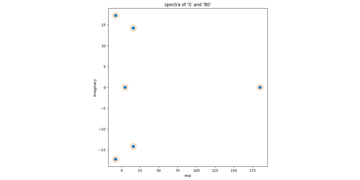
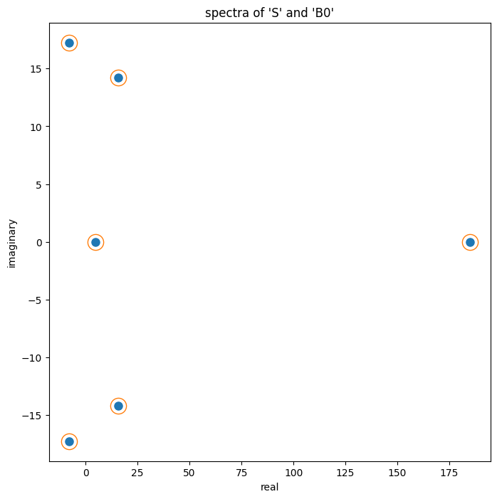
array([185.029 +0.j , -8.052+17.257j, -8.052-17.257j, 15.726+14.192j, 15.726-14.192j, 4.623 +0.j ])Finally, we'll show numerically that S and
B0 have the same eigenvalues. Again, this should be true
given that they S and B0 are similar to each
other.
# similar matrices have the same eigenvalues: compare the spectra
eb = np.linalg.eigvals(B0)
es = np.linalg.eigvals(S)
import matplotlib as mpl
import matplotlib.pyplot as plt
colors = [c['color'] for c in mpl.rcParams['axes.prop_cycle']]
fig = plt.figure(figsize = (8,8))
ax = fig.gca()
ax.plot(np.real(eb), np.imag(eb), ls="none", marker="o", ms = 8, color = colors[0])
ax.plot(np.real(es), np.imag(es), ls="none", marker="o", ms = 16, color = "none", markeredgecolor = colors[1])
ax.set_xlabel("real")
ax.set_ylabel("imaginary")
ax.set_title("spectra of 'S' and 'B0'")
ax;
