
Dustin Lennon
Applied Scientist
dlennon.org
Probabilistic Performance Guarantees for Oversubscribed Resources
This paper constructs a model for shared resource utilization, determines stochastic bounds for resource exhaustion, and simulates results.
Dustin Lennon
November 2012
https://dlennon.org/20121115_over
This work was originally published as an Inferentialist white paper.
Introduction
Introduction
A friend, also an employee at a large, Seattle-area company, recently approached me with the following problem. Suppose we wanted to oversubscribe the shared resources that we lease to our customers. We’ve noticed that loads are often quite low. In fact, loads are so low that there must be a way to allocate at least some of that unused capacity without generating too much risk of resource exhaustion. If we could manage to do this, we could provide service to more people at a cheaper cost! Sure, they might get dropped service on rare occasions, but anyone that wasn’t satisfied with a soft guarantee could still pay a premium and have the full dedicated resource slice to which they may have become accustomed. This seemed like a tractable problem. So after closing out the bar tab, I went home and sketched out the ideas for this paper on my markerboard.
Here, we propose a mathematical framework for solving a very simple version of the problem described above. It provides intuitive tuning parameters that allow for business level calibration of risks and the corresponding reliability of the accompanying service guarantees.
After developing the mathematical framework, we put it to work in a simulation context of customer usage behavior. In this experiment, most customers use only a fraction of the resource purchased, but there is a non-negligible group of “power” users that consume almost all of what they request. The results are rather striking. Compared to the dedicated slice paradigm, resource utilization in the oversubscribed case increases by a factor of 2.5, and more than twice as many customers can be served by the same, original resource pool.
The methodology is easily extended to the non-IID case by standard modifications to the sampling scheme. Moreover, even better performance will be likely if a customer segmentation scheme is incorporated into the underlying stochastic assignment problem.
Mathematical Formulation of the Problem
Mathematical Formulation of the Problem
Suppose individual \(i\) consumes \(Y_i\) units of the resource where \(Y_i\) is a random variable taking values in \(\left[0,c_i\right]\). Thus, individual \(i\) has paid for access to \(c_i\) units but consumes some unknown quantity less than or equal to \(c_i\).
Let \(s_n = \sum_{i=1}^n c_i\), and \(T_n = \sum_{i=1}^n Y_i\) be the total resource purchased and total resource consumed respectively. \(T_n\) must, necessarily, take values in \(\left[0, s_n\right]\). Without loss of generality, we can assume that the resource is exhausted when \(T_n > 1\).
For a given \(n\), choose an acceptable \(\varepsilon\), the risk tolerance for resource exhaustion, such that
\[ \begin{equation} \Pr \left[ T_n > 1 \right] \leq \varepsilon \label{objfn} \end{equation} \]
i.e., the probability of resource exhaustion is less than or equal to \(\varepsilon\).
Then we seek a solution to the following:
\[ \begin{equation} N_{opt} = \argmax_n \left\{ n : \Pr \left[ T_n > 1 \right] \leq \varepsilon \right\} \end{equation} \]
Namely, find the largest \(n\) that doesn’t violated the stated risk tolerance.
In order to obtain \(N_{opt}\), we need to compute an estimate of the objective function,
\[ p_n \equiv \Pr \left[ T_n > 1 \right] \]
The most straightforward approach is to takes samples from the usage distribution. A single sample, say the \(k^{th}\) one of \(K\) total, will be comprised of \(n\) observations and will give rise to the following statistics:
\[ \begin{align} t_k & = \sum_{j=1}^n y_{kj} \label{onesample} \\ b_k & = \mathbb{I}\left( t_k > 1 \right) & \sim & \Bern (p) \label{indicator} \\ c & = \sum_{k=1}^K b_k & \sim & \Bin (p, K) \label{bin} \end{align} \]
where these statistics are characterized by the usual distributions.
Note that \(p\) is tacitly a function of the population of interest from which the \(K\) samples are chosen. It is worth keeping in mind that this population should remain constant across the \(K\) samples. In the current use case, one could imagine different populations corresponding to computational use, web site hosting, etc, or even blends of these. In fact, blends will be particularly useful when dealing with the stochastic assignment problem that would arise when needing to match new users to existing, active resources.
The plan, then, will be to compute a sequence of estimates, increasing \(n\) until we find that we have violated the risk tolerance. At each iteration, take \(K\) samples of size \(n\) and compute the statistics given in Equations \(\ref {onesample}\), \(\ref{indicator}\) and \(\ref{bin}\).
The key step is to define a stopping criterion that gives us control over the probability that we accept a non-violation when, in fact, the risk tolerance probability was exceeded. This is accomplished by choosing a threshold \(c^*\) such that, if we observe \(c > c^*\) we reject the hypothesis that \(p_n\) is less than \(\varepsilon\). In particular, we choose \(\alpha\) such that
\[ \begin{equation} \Pr \left[ C \leq c^*; p > \varepsilon \right] \leq \alpha \label{criterion} \end{equation} \]
Equation \(\ref{criterion}\) should be interpreted as establishing a bound on our willingness to be wrong in the following sense: with probability \(\alpha\), we will incorrectly identify \(n\) to be within risk tolerance when, in fact, this is not the case. So, \(\varepsilon\) and \(\alpha\) are business level decisions. \(\varepsilon\) is the guarantee on the frequency of resource exhaustion and \(\alpha\) is how confident we are that such a guarantee can be made.
The context implies a need for estimates to be conservative; avoiding resource exhaustion is certainly preferable to customer fallout from consistently missing resource guarantees. To that end, note that it is sufficient to enforce the following:
\[ \begin{align} \Pr \left[ C \leq c^*; p > \varepsilon \right] & \leq \Pr \left[ C \leq c^*; p = \varepsilon \right] \notag\\ &\leq \alpha \label{suffcriterion} \end{align} \]
Effectively, we only need to consider Equation \(\ref{criterion}\) in the most difficult case, namely when \(p = \varepsilon\). See Table 1 for calculations of \(c^*\) when \(\alpha = 0.05\) and \(\varepsilon = 0.01\). For a collection of \(K\) samples, the value of \(c^*\) would be the maximum number of resource exceedences allowed in order to give an \(\alpha\)-level guarantee that resources exceed tolerance less than \(\varepsilon\) percent of the time.
Simulation Example
Simulation Example
Without real data, the best that can be done is through simulation. We assume the following:
- Each user is sold access to a 10% slice of a given resource.
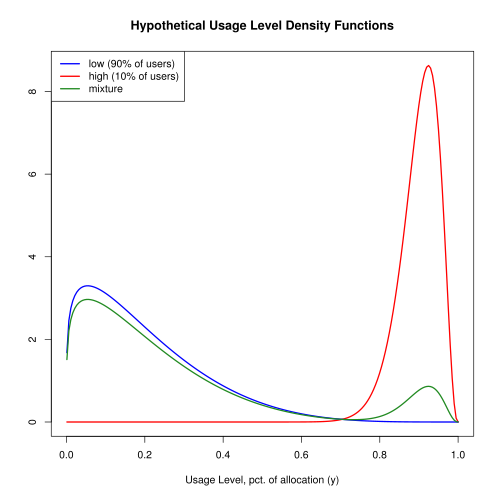
- The usage distribution is a mixture of beta distributions. 90% of users have low resource needs, consuming an average of 20% of their allocated slice. The remaining 10% of users have high resource needs and, on average, consume 90% of their allocation.
Figure 1 shows the probability density functions.
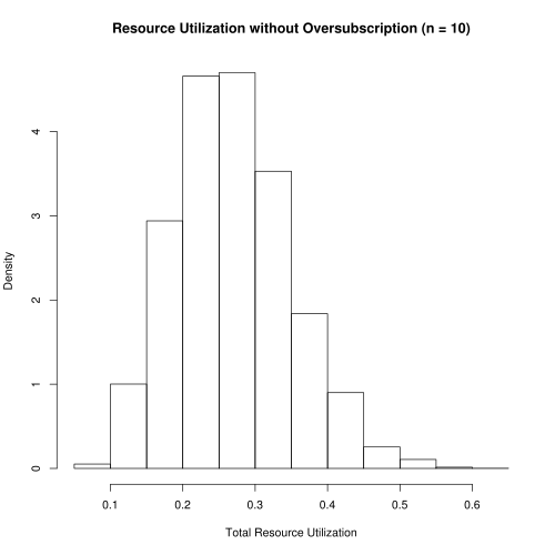
For a resource that does not allow oversubscription, our scenario would allow 10 users to share the resource. A histogram (Figure 2) of usage levels shows that the this resource is woefully underutilized. The guarantee of no resource exhaustion means that we sacrifice 74% of potential resource utilization.
Next, we explore the potential benefits of allowing oversubscription. For a sequence of increasing \(n\) and taking \(K = 10000\), we simulate \(K\) samples, each of size \(n\) drawn from the mixture distribution. For each sample, we compute \(c\) and compare to \(c^*\). The first \(n\) for which \(c > c^*\) is the stopping point.
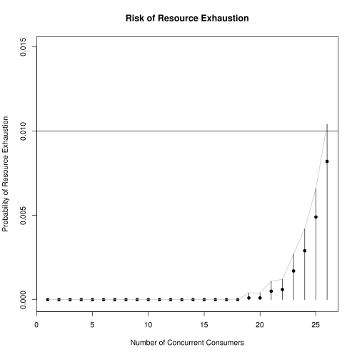
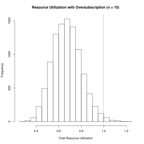
The results in Figure 3 show that the optimal \(n\) that enforces our risk tolerance is \(N_{opt} = 25\). Resource utilization under this scheme is shown in Figure 4 where median resource utilization is now at 66.7%. The gray, vertical line shows the 99% quantile is .994, just shy of 1. This is exactly what we would hope: 99% of the time, resource utilization is less than 0.994. Thus, we can more than double the number of happy users while substantially increasing resource utilization.
In Figure 3, the confidence region reports the \(1 - \alpha\) quantile (divided by \(K\)) of a random variable distributed as \(\Bin(\hat{p}, K)\) where \(\hat{p}\) is the MLE. This is a one-sided confidence interval and based on the exact binomial distribution rather than a normal approximation.
Further Development
Further Development
Changing the sampling scheme to account for live data should be straightforward. Moreover, this scheme could easily be adapted to handle different usage populations. For example, the simplest scenario might be to use a classification engine to identify which usage distribution might best apply to a new customer entering the system.
A more interesting use case of the methodology described here would be as a component of an algorithm that matches new customers to resources already under load. This is a non-trival, stochastic optimal packing problem and would certainly be an interesting project with which to get involved.