Agenda
- Loans 101
- Survival Analysis
- Metrics
- Lending Club
- Machine Learning
- Summary
Loans 101
Loans 101
From the lender's perspective:
- $P_0$, initial investment (dollars out)
- $c$, sequence of payments (dollars in)
- $r$, interest rate (annualized)
- $T$, term of the loan (e.g., 36 months)
- arbitrage: these two cash flows must be equivalent
However, this isn't immediate:
$$ \begin{align*} P_0 \utif^ T \ne c T \end{align*} $$Loans 101: Amortization
The resolution is straightforward:
$P_0$ is lent at time 0.
$P_1$ = $\utif P_0 - c \qquad$ At time 1, $\utif P_0$ is owed and $c$ is paid.
Recursing,
$$ \begin{align*} P_k & = \utif P_{k-1} - c \\ & = \utif \left[ \utif P_{k-2} -c \right] - c \\ & = \utif^k P_0 - c \sum_{i=0}^{k-1} \utif^i \end{align*} $$At time $T$, $P_T = 0$: the loan is paid off.
Loans 101: An arbitrage condition
$P_T = 0$ implies:
$$ \begin{equation*} \utif^T P_0 = c \sum_{i=0}^{T-1} \utif^i \end{equation*} $$Note, each payment must be reinvested.
Implications
- Positions may need to be unwound.
- Any risk persists with each reinvestment.
- Survival analysis "makes sense."
- Generalizations exist for arbitrary time steps, arbitrary payments.
- Internal Rate of Return
Survival Analysis
Survival Analysis: Kaplan Meier
Survival Analysis: Notation
$$ \begin{align*} \widehat{\mathcal{F}}(y) & = \prod_{i:t_i < y} \left( 1 - \hat{h}_i \right) \\ & = \prod_{i:t_i < y} \left( 1 - \frac{a_i}{r_i} \right) \end{align*} $$- $r_i$ the count of units not yet failed or censored at $t_i$, the "risk set"
- $a_i$ is the count of units that fail in $[t_i, t_{i+1})$
- discrete accounting at fixed times; e.g., end of month
Survival Analysis: Definitions
$$ \begin{align*} \mathcal{F}(y) & = \prp{Y \geq y} & \mbox{survival probability} \\ h(y) & = \underset{\Delta \to 0}{\lim} \prp{ y\leq Y < y + \Delta \vert Y \geq y} & \mbox{continuous hazard} \\ & = f(y) / \mathcal{F}(y) \\ h_k & = \prp{ Y = t_k \vert Y \geq t_k } & \mbox{discrete hazard} \\ H(y) & = \int_0^y h(u) du & \mbox{integrated hazard function} \end{align*} $$Parametric modeling is often via the hazard function.
Survival Analysis: Likelihood
Add in censoring:
$d_i = 1$ indicates an observation, $y_i$, is an uncensored failure time; $d_i = 0$, a censored failure time
$$ \begin{align*} l(\theta) & \equiv \sum_{i \in \mathcal{U}} \log f(y_i; \theta) + \sum_{i \in \mathcal{C}} \log \mathcal{F}(y_i) \\ \end{align*} $$When failure is possible only at discrete times,
- $f(y_i)$ and $\mathcal{F}(y_i)$ have telescoping expansions in terms of $h_k$ and $(1-h_k)$; and
- apply a "ragged pivot": aggregate terms over time instead of over unit
Survival Analysis: Modeling
Non-parametric $h_k$
Set $\frac{\partial l(\theta)}{\partial h_k} = 0$ to recover Kaplan-Meier estimator.
Parametric $h_k(\theta)$
If discretized in time:
- Likelihood is a collection of binomial distributions with denominator $r_k$
- Model probabilities are derived via integrated hazard function
Survival Modeling: Hypothesis testing
For each $t_k$, a 2 by 2 contingency table:
| Group A | Group B | Total | |
|---|---|---|---|
| failed | \begin{equation*} a_{k,1} \end{equation*} | $a_{k,2}$ | \begin{equation*} a_{k,1} + a_{k,2} \end{equation*} |
| survived | \begin{equation*} r_{k,1} - a_{k,1} \end{equation*} | \begin{equation*} r_{k,2} - a_{k,2} \end{equation*} | \begin{equation*} (r_{k,1} + r_{k,2}) - (a_{k,1} + a_{k,2}) \end{equation*} |
| total | \begin{equation*} r_{k,1} \end{equation*} | \begin{equation*} r_{k,2} \end{equation*} | \begin{equation*} r_{k,1} + r_{k,2} \end{equation*} |
Test statistic under null hypothesis is hypergeometric:
$$ A_{k,1} \sim \frac{ {{a_{k,1} + a_{k,2}} \choose a_{k,1}} {{(r_{k,1} + r_{k,2}) - (a_{k,1} + a_{k,2})} \choose {r_{k,1} - a_{k,1}}} } { r_{k,1} + r_{k,2} \choose r_{k,1} } $$Log rank statistic: aggregate across the time index, $\mathcal{T}$: $$ Z = \frac{ \sum_{k \in \mathcal{T}} (A_{k,1} - \Ev{A_{k,1}}) }{ \sqrt{ \sum_{k \in \mathcal{T}} \Var{A_{k,1}} } } $$
Metrics
Metrics: Internal rate of return
For a cash flow with no risk of default, IRR is the $r$ that satisfies the earlier arbitrage condition:
$$ \begin{align*} \utif^T P_0 = c \sum_{i=0}^{T-1} \utif^i \end{align*} $$We write the present value of the cash flow as
$$ \begin{align*} P_0 = \frac{1}{\utif}c + \frac{1}{\utif^2}c + \cdots + \frac{1}{\utif^T}c \end{align*} $$and the idea is to appropriately discount each future installment.
Metrics: stochastic discount factors

Let $W_T^{(0)}$ be a portfolio with present value \$1; annualized interest rate, $r$; an installment of $f = c / P$, and $T$ payments remaining.
arbitrage requirement
$$ \begin{align*} \Ev{ W_T^{(0)} } & = \Ev{ D_{1,0} \left( W_{T-1}^{(0)} + f W_{T}^{(1)} \right) } \\ \end{align*} $$Metrics: arbitrage requirement
$$ \begin{align*} \Ev{ W_T^{(0)} } & = \Ev{ D_{1,0} \left( W_{T-1}^{(0)} + f W_{T}^{(1)} \right) } \\ & = \Evk{ D_{1,0} \left. \left( W_{T-1}^{(0)} + f W_T^{(1)} \right) \right\vert Y^{(0)} \geq 1 } \prp{ Y^{(0)} \geq 1 } + 0 \\ & = \frac{ \prp{ Y^{(0)} \geq 1 } }{ \utif } \left\{ \Evk{ \left. W_{T-1}^{(0)} \right\vert Y^{(0)} \geq 1 } + f \Ev{ W_T^{(1)} } \right\} \\ & = d_{1,0} \Evk{ \left. W_{T-1}^{(0)} \right\vert Y^{(0)} \geq 1 } + d_{1,0} f \Ev{ W_T^{(1)} } \end{align*} $$We can apply the above argument recursively:
$$ \begin{align*} 1 & = \Ev{ W_T^{(0)} } \\ & = d_{1,0} f + d_{2,1} d_{1,0} f + \cdots + \left( d_{T,T-1}\cdots d_{1,0} \right) f \end{align*} $$yielding the risk-neutral discount terms
$$ d_{k,0} = d_{k,k-1}\cdots d_{1,0} = \frac{ \prp{ T^{(0)} \geq k } }{ \utif^k } $$Metrics: Risk neutral IRR
We can now meaningfully compute a risk-neutral IRR, $r^*$, for the weighted cash flow:
$$ \begin{align*} P_0 = \frac{\prp{ Y^{(0)} \geq 1 } }{\rnutif}c + \frac{\prp{ Y^{(0)} \geq 2}}{\rnutif^2}c + \cdots + \frac{\prp{ Y^{(0)} \geq T}}{\rnutif^T}c \end{align*} $$Metrics: Probability of repayment
Trivial from KM curve, $\prp{ Y \geq T }$
Potentially useful as:
- an ethical lending constraint;
- a component of a credit score; e.g., the maximal risk-neutral IRR on a loan amount set to 10% of income that has at least a 95% chance of repayment
Lending Club
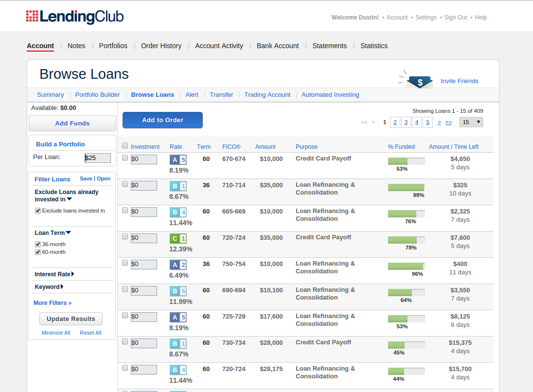
Lending Club: Covariate set, at origination
| column | description |
|---|---|
| loan-amnt | loan amount requested |
| funded-amnt | loan amount funded |
| int-rate | interest rate on loan |
| installment | monthly payment |
| grade | loan quality grade |
| sub-grade | loan quality subgrade |
| purpose | loan category: DEBT-CONSOLIDATION, MEDICAL, ETC. |
| emp-length | employment length |
| home-ownership | home ownership status: RENT, OWN, MORTGAGE, OTHER |
| annual-inc | self reported annual income |
| is-inc-v | income verified |
| fico | FICO score |
| dti | debt to income ratio |
| earliest-cr-line | date of earliest reported credit line |
| open-acc | number of open credit lines |
| revol-bal | total credit revolving balance |
| revol-util | percent credit used |
| total-acc | total number of credit lines in credit file |
| delinq-2yrs | number of 30+ days past-due incidences of delinquency in credit |
| inq-last-6mths | number of inquiries by creditors in the past 6 months |
| mths-since-last-delinq | months since the borrower’s last delinquency |
Lending Club: Covariate set, post-origination
| column | description |
|---|---|
| loan-status | current status of the loan: Charged Off, Current, Fully Paid |
| total-rec-int | interest received to date |
| total-rec-prncp | principal received to date |
| total-rec-late-fee | late fees received to date |
| out-prncp | remaining outstanding principal for total amount funded |
| total-pymnt | payments received to date for total amount funded |
| last-pymnt-d | last date payment was received |
| next-pymnt-d | next scheduled payment date |
| pymnt-plan | indicates if a payment plan is in place for the loan |
Lending Club: Challenges
The full cash flow is unavailable. For post-origination, on the day of data collection, we know only:
- last and next payment dates
- total principal, interest, and fees paid out
- loan status: current, paid, late, very late, charged off
no visibility into timeliness or completeness of payments
Difficult to establish a time of default or assess prepayment risk
"""
  Three estimators of loan length:
    a. last recorded payment        -- "dur_last_pymnt_date"
    b. number of installments paid  -- "dur_total_installment"
    c. interest paid out            -- "dur_total_interest"
"""
examples
| charged off | prepayment | standard | malformed loan | |
|---|---|---|---|---|
| loan_amnt | 1800 | 20000 | 18000 | 7500 |
| int_rate | 11.89 | 11.78 | 14.72 | 13.8 |
| term | 36 | 36 | 36 | 36 |
| installment | 59.7 | 662.19 | 621.52 | 236.86 |
| issue_d | 2008-12-05 | 2008-12-05 | 2010-08-06 | 2008-09-26 |
| last_pymnt_d | 2010-03-30 | 2010-09-08 | 2013-08-22 | 2011-09-29 |
| total_pymnt | 673.21 | 23036.2 | 22368.3 | 8526.93 |
| total_rec_prncp | 436.01 | 20000 | 18000 | 6950 |
| full_interest | 349.2 | 3838.84 | 4374.72 | 1026.96 |
| total_rec_int | 160.99 | 3003.13 | 4368.26 | 1576.93 |
| loan_status | Charged Off | Fully Paid | Fully Paid | Fully Paid |
| dur_last_pymnt_date | 15.7703 | 21.0928 | 36.5346 | 36.0747 |
| dur_total_installment | 11.2765 | 34.7879 | 35.9896 | 35.9999 |
| dur_total_interest | 10.134 | 19.9876 | 35.1976 | 24.7193 |
"""
  ETL / data cleaning
"""

# Loan parameters must be conformal; those that aren't destroy the KM curves
# *** 299 records removed ***
data['is_valid'] = False
for i,record in enumerate(data.itertuples()):
    data.loc[record.Index,'is_valid'] = util.is_valid_loan(record)
data    = data.loc[ data.is_valid ].copy()

# Only focus on 'Charged Off' and 'Fully Paid' loans
# *** 18 more records removed ***
data    = data.loc[ data.loan_status.isin(['Charged Off', 'Fully Paid'])].copy()

# Any record where more principal is paid back than is borrowed is structurally wrong;
# *** 350 more records removed ***
data    = data.loc[ data.total_rec_prncp <= data.loan_amnt ].copy()

# Any record where the totals don't add up to their components is badly formed;
# *** 642 more records removed ***
lit     = data.total_rec_prncp + data.total_rec_int + data.total_rec_late_fee
agt     = data.total_pymnt
data    = data.loc[ np.abs(lit - agt) < 1 ].copy()

# Group the lower performing loans together
lgi     = data.grade.isin(['E','F','G'])
data.loc[lgi,'grade'] = 'E+'
Machine Learning
Machine Learning: Where to start?
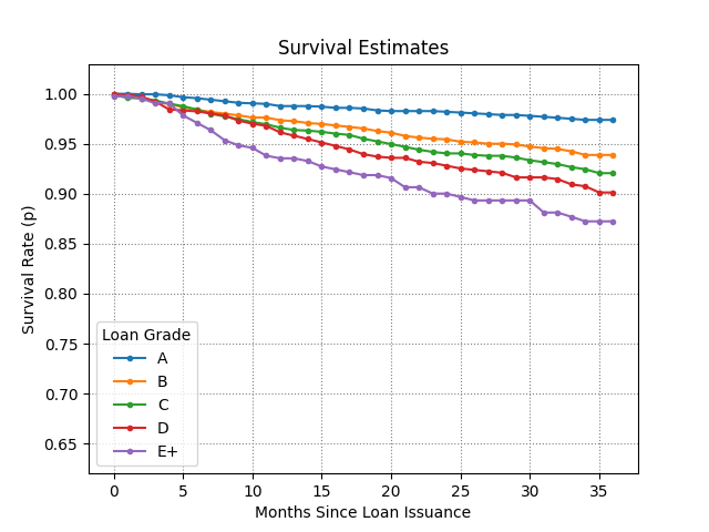
- We can estimate survival curves for sets of loans (Kaplan Meier).
- We can quantify the difference equivalence classes (log rank statistic).
- We don't want to work too hard.
Random forest
- Split on the log rank statistic.
- Obtain bootstrap estimates (and variances) of our metrics.
- Easily handle categorical variables and outliers.
Machine Learning: Random forest, construction
Take B bootstrap samples of size N.
For each bootstrap sample, build a partitioning tree, $T_b$:
- Select $m < p$ variables as split candidates
- For each split candidate, determine a set of split values
- Compute best split
- Partition the node and recurse
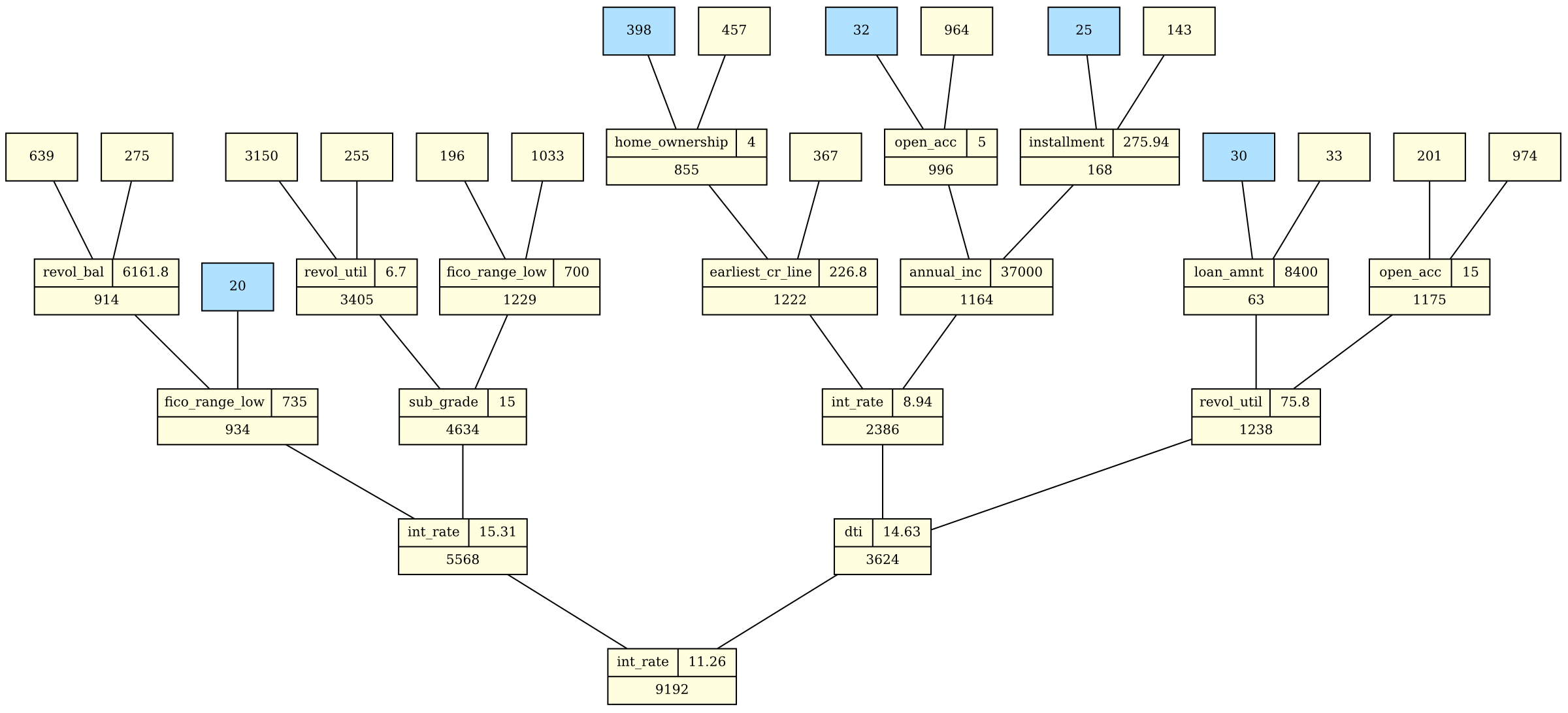
- blue nodes are terminal nodes; size, or statistically homogeneous
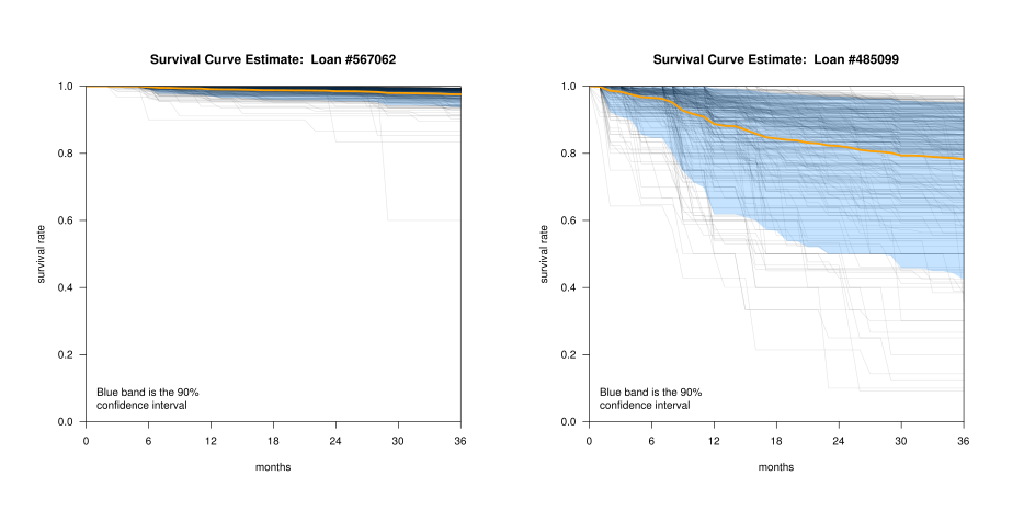
Machine learning: Random forest, scoring
Score a loan, $i$, via OOB tree set, $\mathcal{T}_i$:
- For each $t \in \mathcal{T}_i$, find the leaf node that would have contained $i$
- Compute any summary statistics, $S_{i,t}$
- $\mathcal{X}_i = \left\{ S_{i,t} : t \in \mathcal{T}_i \right\}$ is a predictive distribution of the summary statistics associated with loan $i$
Machine Learning: Random forest, survival curves
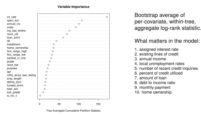
Machine Learning: Variable importance
Summary
Summary: Using an investor-trained model
- Term and loan amounts: likely fixed.
- One remaining free parameter: interest rate or installment.
Analogous to profile likelihood / parameter scan:
- Partition the covariate vector: loan- and user-specific components
- Replace loan-specific components by a set of loan parameters (levels)
- For each query, use the corresponding survival curve to infer IRR, probability of repayment.